Add Column Sparklines To Cells F2 F11
Breaking News Today
Mar 22, 2025 · 5 min read
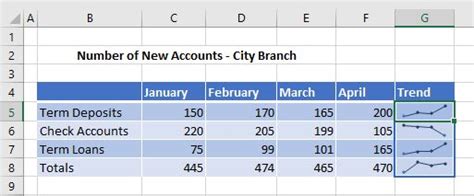
Table of Contents
Adding Sparklines to Cells F2:F11 in Excel: A Comprehensive Guide
Sparklines are miniature charts that fit within a single cell, providing a visual summary of data trends. They're a powerful tool for quickly understanding data patterns without cluttering your spreadsheet with large charts. This guide will walk you through adding sparklines to cells F2:F11 in Excel, covering various sparkline types, customization options, and troubleshooting tips.
Understanding Sparkline Types
Excel offers three primary sparkline types:
- Line: Shows data trends over time or across categories. Ideal for highlighting highs, lows, and overall direction.
- Column: Represents data as vertical columns, excellent for comparing values across different periods or groups.
- Win/Loss: Displays wins (positive values) as green columns and losses (negative values) as red columns. Useful for visualizing performance data.
For this tutorial, we'll primarily focus on adding column sparklines to cells F2:F11, but the principles can be easily applied to other types.
Step-by-Step Guide: Adding Column Sparklines to Cells F2:F11
Before you begin, ensure you have data in cells that will feed your sparklines. Let's assume your data for the sparklines resides in cells A2:A11. These values will be the source data for the sparklines in cells F2:F11.
1. Select the Sparkline Range:
Click on cell F2, then drag your mouse to select the range F2:F11. This is where your sparklines will be displayed.
2. Access the Sparklines Feature:
Navigate to the "Insert" tab on the Excel ribbon. In the "Charts" group, you should see the "Sparklines" button. Click it.
3. Choose the Sparkline Type:
A small window will appear, prompting you to select a sparkline type. Choose "Column" from the dropdown menu.
4. Specify the Data Range:
The next section requires you to specify the data range that will populate your sparklines. This is crucial. In the "Data Range" field, enter A2:A11 (or the actual range containing your data). Make sure the range aligns correctly with the selected sparkline range (F2:F11). This step is where many users encounter issues, so double-check your data range.
5. Location (Optional):
The "Location" field usually defaults to "Right" or "Below" the selection. Since you have already selected the range F2:F11, this should be correct. Leaving this as the default setting usually works best for this instance.
6. Click "OK":
Once you've confirmed the data range and location, click "OK." Excel will generate column sparklines in cells F2:F11, visually representing the data in cells A2:A11.
Customizing Your Column Sparklines
The default sparklines are functional, but often benefit from customization to enhance readability and visual appeal. Let's explore several customization options:
1. Modifying Sparkline Appearance:
- High Point: By default, the highest data point is marked. You can customize the marker style, color, and size to make it more prominent. Explore the sparkline design options for this.
- Low Point: Similarly, the lowest point is usually marked. Adjust its appearance to match the high point or use different styles to highlight contrast.
- Negative Points: If your data includes negative values, you can customize how they are visually represented (e.g., different color, marker).
- Axis: You can choose to display a vertical axis or not; this can greatly impact the appearance depending on your data.
- Markers: Explore different marker options – circles, squares, or none.
- Color: Choose the fill color to enhance the visual impact.
2. Advanced Customization with "Design" Tab:
Once you've created your sparklines, a new "Sparkline Tools" tab will appear in the ribbon. This tab houses various options for design and formatting. The “Design” tab offers advanced customizations:
- Change Chart Type: If you decide you'd prefer a different sparkline type (line or win/loss), you can easily change it here.
- Show High Point: Turn this on or off to emphasize peak performance.
- Show Low Point: Emphasize the lowest data point.
- Show Markers: Display markers for individual data points (useful for emphasizing specific points of interest).
- Show First Point: Useful for highlighting starting points.
- Show Last Point: Highlights ending values.
- Show Negative Points: Visualize negative values distinctly.
- Show Axis: Add or remove axis markers for better readability depending on the data context.
- Horizontal Axis: Control the visible axis on the sparkline.
3. Formatting Options:
The "Format" tab provides further options:
- Fill: Adjust the fill color and pattern of the columns.
- Border: Add borders to individual columns for better distinction.
- Size: While you can't dramatically change the size within the cell, you can make slight adjustments.
- Data Labels: Add data labels above or below the columns.
Troubleshooting Common Sparkline Issues
- #NAME? Error: This often indicates an incorrect data range reference. Double-check the data range specified in the Sparkline options.
- Blank Sparklines: This usually stems from empty cells in the data range. Ensure your source data cells (A2:A11 in our example) contain numerical values.
- Inconsistent Sparkline Appearance: This might result from mixed data types in your source data (e.g., numbers and text). Confirm your data range contains only numerical values.
Leveraging Sparklines for Effective Data Visualization
Sparklines are a powerful tool for adding concise visual summaries directly within your spreadsheet. By strategically using different sparkline types and customization options, you can create informative dashboards that clearly communicate data trends without needing separate charts. Consider these points:
- Data Clarity: Use sparklines to highlight key trends and patterns within larger datasets.
- Contextual Understanding: Ensure the underlying data is readily accessible for a complete understanding of the sparkline's meaning.
- Visual Appeal: Choose a consistent color scheme and customize sparkline elements to maintain visual appeal.
- Strategic Placement: Place sparklines next to relevant data to streamline information access.
Beyond the Basics: Advanced Sparkline Applications
Once you've mastered the basics, explore more advanced applications:
- Conditional Formatting: Combine sparklines with conditional formatting to highlight specific data points based on thresholds.
- Data Series Combinations: Use multiple data series to represent different aspects of your data within one sparkline.
- Interactive Sparklines: Although not a native feature, you can create interactive effects using VBA scripting.
By implementing the steps outlined above, diligently reviewing your data range, and exploring customization features, you can effectively utilize sparklines to transform your Excel spreadsheets into dynamic and insightful visual representations of your data. Mastering sparklines is a significant step towards efficient data management and communication. Remember to always double-check your data range and utilize the customization options to create easily interpretable and visually appealing sparklines.
Latest Posts
Latest Posts
-
Treatment With Continuous Positive Airway Pressure Quizlet
Mar 24, 2025
-
What Is A Sign Of Alcohol Poisoning Quizlet
Mar 24, 2025
-
Ati Test Taking Strategies Seminar Posttest Quizlet
Mar 24, 2025
Related Post
Thank you for visiting our website which covers about Add Column Sparklines To Cells F2 F11 . We hope the information provided has been useful to you. Feel free to contact us if you have any questions or need further assistance. See you next time and don't miss to bookmark.
