Which Graph Represents The Following Piecewise Defined Function
Breaking News Today
Mar 24, 2025 · 6 min read
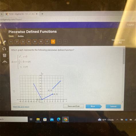
Table of Contents
Which Graph Represents the Following Piecewise Defined Function? A Comprehensive Guide
Piecewise functions, those mathematical chameleons that change their form depending on the input, can sometimes be tricky to visualize. Understanding how to represent them graphically is crucial for grasping their behavior and applying them in various fields like engineering, economics, and computer science. This article will delve deep into the process of identifying the correct graph for a given piecewise defined function, providing you with the tools and knowledge to tackle any such problem with confidence.
Understanding Piecewise Defined Functions
A piecewise function is defined by multiple sub-functions, each applicable over a specific interval of the domain. The key is to understand the domain restriction for each sub-function. This restriction dictates which part of the graph the sub-function contributes to. The function's overall graph is a compilation of these individual sub-graphs. A typical representation looks something like this:
f(x) = {
    g(x),  if a ≤ x < b
    h(x),  if b ≤ x ≤ c
    i(x),  if x > c
}
Here, g(x), h(x), and i(x) are different functions, each active only within their specified domain intervals: [a, b), [b, c], and (c, ∞), respectively. The parentheses and brackets indicate whether the endpoints are included or excluded from the interval.
Step-by-Step Guide to Graphing Piecewise Functions
Let's outline a systematic approach to graphing these functions, ensuring accuracy and preventing common pitfalls:
1. Analyze Each Sub-function Individually:
Begin by examining each sub-function separately. Determine its type (linear, quadratic, absolute value, etc.). This will give you an idea of its general shape. For instance:
- Linear Function (e.g., y = mx + c): A straight line with slope
mand y-interceptc. - Quadratic Function (e.g., y = ax² + bx + c): A parabola that opens upwards if
a > 0and downwards ifa < 0. - Absolute Value Function (e.g., y = |x|): A V-shaped graph with a vertex at the origin.
2. Determine the Domain Restrictions:
Carefully note the domain restrictions for each sub-function. These are crucial for determining which portion of the graph each sub-function contributes. Pay close attention to whether the endpoints are included (using square brackets [ and ]) or excluded (using parentheses ( and )). This impacts the continuity of the graph.
3. Plot Key Points:
For each sub-function, determine and plot key points. These points will help you accurately sketch the graph within the specified domain. For linear functions, two points are sufficient. For quadratic functions, the vertex and a few other points are helpful. For more complex functions, consider using a table of values.
4. Connect the Points:
Connect the plotted points for each sub-function, remembering the domain restriction. Do not extend the graph beyond the boundaries defined by the domain.
5. Check for Continuity:
Examine the graph at the boundaries between sub-functions. If the endpoints are included in both adjacent intervals, ensure there is no break in the graph. A "jump" or discontinuity indicates an error in either the plotting or the understanding of the piecewise function.
6. Verify with a Calculator or Software:
While manual graphing is essential for understanding, it's always wise to verify your results using a graphing calculator or software like Desmos or GeoGebra. These tools provide accurate visualizations and can help identify any mistakes.
Common Mistakes to Avoid
- Ignoring Domain Restrictions: This is the most common mistake. Always carefully consider the domain of each sub-function. Ignoring this leads to incorrect graphs that extend beyond the specified intervals.
- Incorrect Endpoint Handling: Pay close attention to whether the endpoints are included or excluded. A small mistake here can significantly alter the graph's appearance.
- Incorrect Function Interpretation: Misunderstanding the type of sub-function can lead to an incorrect graph shape. Double-check your interpretation of each sub-function before plotting.
- Failing to Check Continuity: The graph may appear correct, but a quick continuity check can reveal errors. Look for jumps or breaks in the graph, especially at the boundaries between intervals.
Examples and Illustrations
Let's illustrate the process with a few examples:
Example 1:
Consider the piecewise function:
f(x) = {
    x + 1, if x < 0
    x² ,  if x ≥ 0
}
Solution:
-
Sub-function Analysis: We have a linear function (
x + 1) and a quadratic function (x²). -
Domain Restrictions:
x + 1is active forx < 0, andx²is active forx ≥ 0. -
Plotting Key Points: For
x + 1, plot points like (-1, 0) and (-2, -1). Forx², plot points like (0, 0), (1, 1), and (2, 4). -
Connecting Points: Draw a line for
x + 1to the left of x = 0 (excluding x = 0) and a parabola forx²starting at x = 0 and extending to the right. Note that the two parts meet at (0,0), even though the line doesn't actually reach the point (0,1). -
Continuity Check: The graph is continuous at x = 0, although it is made up of two separate functions.
Example 2:
Consider the piecewise function:
f(x) = {
    |x|, if x ≤ 2
    4 - x, if x > 2
}
Solution:
-
Sub-function Analysis: An absolute value function (
|x|) and a linear function (4 - x). -
Domain Restrictions:
|x|forx ≤ 2, and4 - xforx > 2. -
Plotting Key Points: For
|x|, plot points like (0, 0), (1, 1), (2, 2). For4 - x, plot points like (2, 2), (3, 1), (4, 0). -
Connecting Points: Draw the absolute value V-shape up to x = 2, and then a decreasing line starting from (2, 2). Note that the point (2,2) is shared between the two sub-functions.
-
Continuity Check: The graph is continuous at x = 2.
Example 3 (Illustrating Discontinuity):
f(x) = {
    x + 2, if x < 1
    x - 2, if x ≥ 1
}
Solution: This example will show a discontinuity. Following the steps above, you'll notice a jump in the graph at x = 1. The left-hand limit approaches 3, while the right-hand limit approaches -1. This is a crucial observation when interpreting piecewise functions.
Conclusion
Mastering the art of graphing piecewise functions is a valuable skill for anyone working with mathematical models. By carefully analyzing each sub-function, understanding domain restrictions, and paying close attention to detail, you can confidently represent these functions graphically and accurately interpret their behavior. Remember to always double-check your work, and don't hesitate to use graphing calculators or software to verify your results. The examples provided highlight the key concepts and common pitfalls, equipping you to tackle a wide range of piecewise function problems with precision and understanding. Remember, practice makes perfect! Work through various examples, experimenting with different function types and domain restrictions to solidify your understanding and build your skills.
Latest Posts
Latest Posts
-
Simulation Lab 4 1 Module 04 Repair A Duplicate Ip Address
Mar 29, 2025
-
When Nucleotides Polymerize To Form A Nucleic Acid
Mar 29, 2025
-
The Average Adult Eats About 4 000 Calories A Day
Mar 29, 2025
-
When Vehicle Wheels Are About To Lock The Abs
Mar 29, 2025
-
The Par Value Per Share Of Common Stock Represents
Mar 29, 2025
Related Post
Thank you for visiting our website which covers about Which Graph Represents The Following Piecewise Defined Function . We hope the information provided has been useful to you. Feel free to contact us if you have any questions or need further assistance. See you next time and don't miss to bookmark.
