A Numerical Outcome Of A Probability Experiment Is Called
Breaking News Today
Mar 20, 2025 · 6 min read
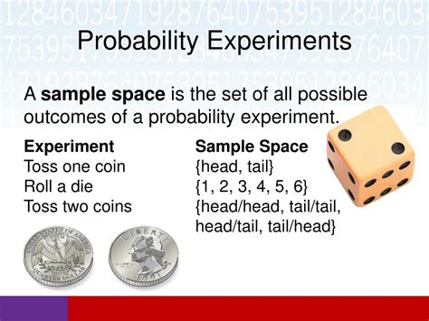
Table of Contents
A Numerical Outcome of a Probability Experiment is Called a Random Variable
Understanding probability experiments and their numerical outcomes is fundamental to various fields, from statistics and data science to finance and game theory. A crucial concept in this understanding is the random variable. This article delves deep into what a random variable is, its types, and how it's used in probability calculations and statistical analysis.
What is a Random Variable?
A numerical outcome of a probability experiment is called a random variable. It's a variable whose value is a numerical outcome of a random phenomenon. In simpler terms, it's a function that maps the outcomes of a probability experiment to numerical values. These values can be discrete (countable) or continuous (uncountable).
Let's break this down further:
-
Probability Experiment: Any process that can produce a well-defined outcome. Examples include flipping a coin, rolling a die, measuring the height of students in a class, or observing the number of cars passing a certain point on a highway within an hour.
-
Outcome: The result of a single trial of a probability experiment. For example, the outcome of flipping a coin could be heads or tails; the outcome of rolling a die could be any number from 1 to 6.
-
Random Variable (X): A numerical representation of the outcome. It assigns a numerical value to each possible outcome of the experiment.
Example:
Consider the experiment of rolling a fair six-sided die. The possible outcomes are {1, 2, 3, 4, 5, 6}. We can define a random variable X as the number rolled. Therefore:
- If the outcome is 1, then X = 1.
- If the outcome is 2, then X = 2.
- And so on...
This simple example showcases the core concept: the random variable transforms qualitative outcomes (heads/tails, 1/2/3/4/5/6) into quantitative data (numerical values) that we can analyze statistically.
Types of Random Variables
Random variables are broadly categorized into two main types:
1. Discrete Random Variables
A discrete random variable can only take on a finite number of values or a countably infinite number of values. These values are often integers, but they don't have to be. The key is that you can count them.
Examples:
- Number of heads in three coin flips: The possible values are 0, 1, 2, and 3.
- Number of cars passing a point in an hour: The values are non-negative integers (0, 1, 2, 3,...).
- Number of defective items in a batch of 100: The values are integers from 0 to 100.
- The outcome of rolling two dice and summing the numbers: Values range from 2 to 12.
Discrete random variables are often associated with probability mass functions (PMFs). A PMF assigns a probability to each possible value of the discrete random variable.
2. Continuous Random Variables
A continuous random variable can take on any value within a given range or interval. The number of possible values is uncountably infinite. You cannot count the values; instead, you measure them.
Examples:
- Height of a person: Height can take on any value within a certain range (e.g., 150cm to 200cm).
- Temperature of a room: Temperature can be any value within a range.
- Weight of an object: Weight can take any value within a certain range.
- Time taken to complete a task: Time can be any value within a given range.
Continuous random variables are often associated with probability density functions (PDFs). A PDF describes the relative likelihood of the random variable taking on a given value. Unlike a PMF which gives the probability of a specific value, the PDF gives the probability density at a specific value. The probability of a continuous random variable taking on any single specific value is actually zero. Instead, we calculate probabilities over intervals.
Probability Distributions
Both discrete and continuous random variables have associated probability distributions. These distributions describe the likelihood of different outcomes.
Probability Mass Function (PMF) for Discrete Random Variables
The PMF, denoted as P(X=x), gives the probability that the discrete random variable X takes on the value x. The sum of probabilities for all possible values of X must equal 1.
Example: Let X be the number of heads obtained in two coin flips. The PMF is:
- P(X=0) = 0.25 (both tails)
- P(X=1) = 0.5 (one head, one tail)
- P(X=2) = 0.25 (both heads)
Note that P(X=0) + P(X=1) + P(X=2) = 1.
Probability Density Function (PDF) for Continuous Random Variables
The PDF, denoted as f(x), describes the relative likelihood of the random variable X taking on a value around x. The probability that X falls within a given interval is given by the integral of the PDF over that interval. The total area under the PDF curve must equal 1.
Example: The normal distribution is a common example of a continuous probability distribution. Its PDF is a bell-shaped curve.
Cumulative Distribution Function (CDF)
The cumulative distribution function (CDF), denoted as F(x), gives the probability that the random variable X is less than or equal to a certain value x. It's defined for both discrete and continuous random variables. For a discrete variable, it's the sum of probabilities up to x. For a continuous variable, it's the integral of the PDF up to x. The CDF is always a non-decreasing function, ranging from 0 to 1.
Expected Value and Variance
The expected value (E[X] or μ) of a random variable is its average value, weighted by the probabilities of its possible values. For a discrete variable, it's the sum of each value multiplied by its probability. For a continuous variable, it's the integral of x times the PDF.
The variance (Var(X) or σ²) measures the spread or dispersion of the random variable around its expected value. A high variance indicates a wide spread, while a low variance indicates values clustered close to the mean. The standard deviation (σ) is the square root of the variance.
Applications of Random Variables
Random variables are essential tools in many areas:
-
Statistical Inference: Random variables are used to model populations and make inferences about them based on sample data. Hypothesis testing, confidence intervals, and regression analysis all heavily rely on random variables.
-
Risk Management: In finance, random variables are used to model asset returns and assess risk. Portfolio optimization and option pricing utilize probability distributions of random variables.
-
Machine Learning: Many machine learning algorithms work with random variables. For example, Bayesian methods use probability distributions to represent uncertainty.
-
Simulation: Random variables are used to generate random numbers in simulations to model real-world systems and predict outcomes. This is used in areas such as queuing theory, traffic flow modeling, and weather forecasting.
-
Quality Control: In manufacturing, random variables are used to assess the quality of products and processes. Control charts and acceptance sampling techniques rely on the understanding of random variables.
Conclusion
Understanding random variables is crucial for anyone working with probability and statistics. The ability to identify whether a variable is discrete or continuous, to understand its probability distribution, and to calculate its expected value and variance are essential skills. The applications of random variables span various disciplines, making them a cornerstone of quantitative analysis in numerous fields. From modeling complex systems to making informed decisions under uncertainty, the power of random variables remains undeniable. This comprehensive overview provides a solid foundation for further exploration of this fundamental concept. Remember to always consider the context of the experiment and the nature of the numerical outcomes when identifying and characterizing a random variable.
Latest Posts
Latest Posts
-
When The Atria Contract Which Of The Following Is True
Mar 21, 2025
-
Unit 4 Progress Check Mcq Part B
Mar 21, 2025
-
Signs And Symptoms Of A Sympathomimetic Drug Overdose Include
Mar 21, 2025
-
Approximately 75 Percent Of Struck By Fatalities Involve
Mar 21, 2025
-
Laura Conocia Bien A Elian Elian Conocia Bien A Laura
Mar 21, 2025
Related Post
Thank you for visiting our website which covers about A Numerical Outcome Of A Probability Experiment Is Called . We hope the information provided has been useful to you. Feel free to contact us if you have any questions or need further assistance. See you next time and don't miss to bookmark.
